Estimated Baseline Hazard Function in R with ggplot2

March 02, 2024

In this tutorial, we will delve into depicting the estimated (cumulative) baseline hazard functions in R using the ggplot2 package. As we observe, a Cox proportional hazard regression comprises two components: a non-specific baseline hazard function of time and a linear predictor in exponential form:

\[\lambda_{i}(t) = \lambda_{0}(t)e^{X_{i}(t) \beta},\]

where \(i\) is the index for a unique patient, \(t\) represents a specific timepoint, \(\lambda_{0}(t)\) is the non-specific baseline hazard function over time, \(X_{i}(t)\) includes covariates for patient \(i\) at time \(t\), and \(\beta\) is a vector of coefficients. Typically, estimated coefficients can be obtained using the coxph() function in the survival package. However, procedures to obtain \(\lambda_{0}(t)\) are less commonly discussed. This is because Cox regression is a semi-parametric model that incorporates a non-parametric component for the baseline hazard function, making it unspecified. Additionally, the estimation of the baseline hazard function is often challenging, and its statistical inference remains mysterious in the cutting-edge research of survival analysis. In comparison, estimating the cumulative (or integrated) baseline hazard function is generally easier than estimating the baseline hazard function. Therefore, we will start our illustration by focusing on the estimation of the cumulative baseline hazard function.

1. Estimator

We begin with a non-parametric estimator, the Nelson-Aalen estimator for the cumulative baseline hazard function. It can be expressed as:

\[\hat{\Lambda}(t) = \sum_{i: t_{i} \leq t} \frac{d_i}{r_{i}},\]

where \(d_i\) is the number of events at time \(t_{i}\), and \(r_{i}\) is the number of patients “at risk” (i.e., under observation) at time \(t_{i}\). More specifically, under counting-process-type expression, it can also be expressed as:

\[\hat{\Lambda}(t) = \int_{0}^{t} \frac{d \bar{N}(s)}{ \sum_{i} \bar{Y}_{i}(s) },\]

where \(d \bar{N}(s)\) is the number of events occurring precisely at time \(s\), and \(\bar{Y}_{i}(s)\) is the number of patients “at risk” at time \(s\). Heuristically, the Nelson-Aalen estimator is a method of moments estimator and can be reasonably considered as a Poisson process at a short time period \(t\). Therefore, its estimated variance can be obtained as

\[\hat{Var}(\hat{\Lambda}) = \sum_{i: t_{i} \leq t} \frac{d_i}{r_{i}^2},\]

where \(r_{i}\) is the number of patients “at risk” (i.e., under observation). The detailed procedure involves measure theory and stochastic process and is quite technical, so we will omit it here. In addition to the Nelson-Aalen estimator, the Breslow estimator for the cumulative baseline hazard function is often used after fitting Cox regression. Essentially, the Breslow estimator aims to estimate a survival function \(S(t)\) and is intricately connected with the cumulative baseline hazard function \(S(t) = e^{- \Lambda(t)}\). As the exponential function is continuous and monotonic, the crucial aspect of the Breslow estimator lies in obtaining the estimate of \(\Lambda(t)\). In general, the Breslow estimator can be expressed as

\[\hat{\Lambda}(t) = \sum_{i: t_{i} \leq t} \frac{d_i}{\sum_{i: t_{i} \leq t} e^{X_{i} \hat{\beta}}},\]

where \(\hat{\beta}\) can be obtained from the maximum partial likelihood estimator. Interestingly, the Breslow estimator is equivalent to the Nelson-Aalen estimator when all covariates are set to zero. Considering the counting-process-type expression, we can rewrite it as follows:

\[\hat{\Lambda}(t) = \sum_{i = 1}^{n} [\int_{0}^{t} \frac{dN_{i}(s)}{\sum_{i = 1}^{n}(Y_{i}(s) e^{X_{i} \hat{\beta}})}],\]

where \(dN_{i}(s)\) indicates if an event happened at time \(s\) for a patient \(i\), \(Y_{i}(s)\) indicates if a patient \(i\) is still under observation at time \(s\), \(n\) is the total number of patients. Therefore, we noticed that

\[\bar{N}(s) = \sum_{i = 1}^{n} N_{i}(s), \quad \bar{Y}_{i}(s) = \sum_{i = 1}^{n} Y_{i}(s).\]

The detailed proof involves the use of Fubini’s theorem to enable the interchangeability of integration and summation, but we will omit it here. Since both estimators are designed for the cumulative (integrated) baseline hazard, if we aim to derive the baseline hazard function \(\lambda_{0}(t)\) from the cumulative baseline hazard \(\Lambda(t)\), we need to take the stepwise discrete-time derivative for the cumulative (integrated) baseline hazard. It is worth noting that, while this approximation may not be very precise, the associated statistical inference (i.e., asymptotics) remains somewhat mysterious. Nevertheless, it serves as an informative tool for visualizing the baseline risk of event occurrence. Sometimes, understanding the behavior of a Cox model in this context can be useful and may be used for comparisons with the incidence rate over time in lots of infectious diseases studies. Particularly, when applying time-dependent covariate or time-varying coefficient Cox models, the visualization of the baseline hazard can convey more information about the underlying behavior of the model. Now, we are moving on to the visualization part.

2. Dataset

The simulated dataset is designed to investigate the risk of secondary infection with various respiratory viruses after the primary rhinovirus infections, representing a type of viral interference. It comprises six columns:

• PID: this is an unique identification for each participants (string);

• start and stop: these two columns represent the counting-process-type of data, where they together define the observation time interval (start, end] (numerical);

• rhinovirusInitial: this is a binary indicator for whether a rhinovirus infection is detected at the end of an observation interval (i.e., 1 for detected and 0 for not detected) (numerical);

• secondInfection: this is a binary indicator for whether other viral infection is detected at the end of an observation interval (i.e., 1 for detected and 0 for not detected) and it is the outcome variable (numerical);

• afterInitialInfection: this is a time-dependent covariate that categorizes an observational interval into four types: no secondary infections, detected secondary infection less than or equal to 90 days after the primary infection, detected secondary infection greater than 90 days but less than or equal to 180 days after the primary infection, and detected secondary infection greater than 180 days but less than or equal to 365 days after the primary infection [4 levels: No, Day <= 90, 90 < Day <= 180, 180 < Day <= 365] (string).

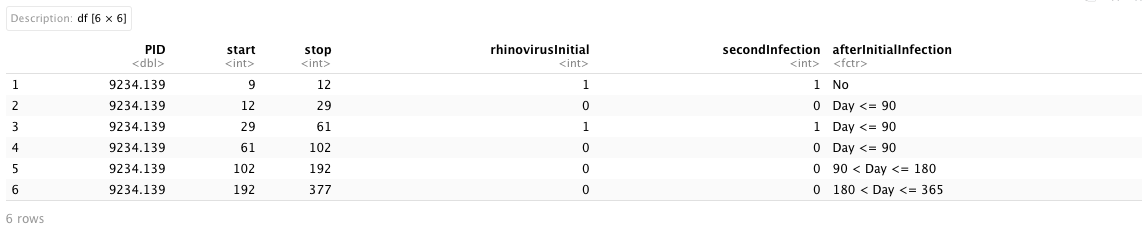
We also assumed that these patients are part of a prospective longitudinal cohort study, ensuring that each patient had at least two observations over the study period. To incorporate the calendar time scale into the modeling procedure, the start and stop time points are adjusted relative to the study’s initialized calendar date.

3. Stepwise discrete-time derivative

Given the awareness that only the cumulative (integrated) baseline hazard can be estimated with valid statistical inference, results from a Cox model in R provide the estimated cumulative baseline hazard function using the Breslow estimator, which is also equivalent to the Nelson-Aalen estimator when all covariates are set to zero. Therefore, we need to create a manual function to calculate the stepwise discrete-time derivative and use it to manually perform the derivative for the estimated cumulative baseline hazard function. The following code snippet is an example of performing the stepwise discrete-time derivative.

finite_differences <- function(x, y) {
  n <- length(x)
  derivativeFunction <- vector(length = n)
  for (i in 2:n) {
    derivativeFunction[i-1] <- (y[i-1] - y[i]) / (x[i-1] - x[i])
  }
  derivativeFunction[n] <- (y[n] - y[n - 1]) / (x[n] - x[n - 1])
  return(derivativeFunction)
}

Since there are multiple code structures that can compute the stepwise discrete-time derivative, we present a self-created version. One may choose any type of stepwise discrete-time derivative function to calculate the derivative.

4. Baseline hazard function

To obtain the estimated baseline hazard function, we first need to construct a Cox model in R. Essentially, we need to utilize the Surv() and coxph() functions from the survival package to construct a Cox model:

• Surv(): it is a function used to create a survival object, typically employed as a response variable in a model formula. It requires to specify several arguments:

  • time and time2: they are used to specify an observation time interval, denoted as (time, time2] = (start, stop]);

  • event: it is used to specify the status indicator, representing a binary event outcome.

• coxph(): it is used to fit a Cox proportional hazards regression model.

We will utilize the Surv() function to set up a survival outcome and employ coxph() to fit a model.

require(survival)
# Fit cox regression
fomula <- Surv(start, stop, secondInfection) ~ afterInitialInfection  # construct formula 
model <- coxph(fomula, cluster = PID, data = Dt)  # due to repeated measurement over time using robust variance (set cluster = PID)
Summary <- summary(model)  # Obtain model summary

# Create coefficient table
resultTable <- cbind(Summary$coefficients, Summary$conf.int[, c('lower .95', 'upper .95')])
round(resultTable, 4)

After fitting the Cox model, we obtained estimated hazard ratios for the time-dependent covariate to evaluate the risk of secondary infections of other viruses after the primary rhinovirus infection. We found that the risk of secondary infections of other viruses within 90 days (HR: 0.58, 95% CI: 0.43, 0.77) and after 180 days but before 365 days (HR: 0.27, 95% CI: 0.18, 0.42) after the primary rhinovirus infection was significantly decreased compared to patients without a primary rhinovirus infection. Although the risk of secondary infections of other viruses after 90 days but before 180 days was not statistically significant, it was still estimated as a decreased risk. These results are consistent with previous research related to the antiviral state after human rhinovirus infection.

Now that we have obtained the fitted Cox model, we are going to derive the estimated cumulative baseline hazard function from this model using the basehaz() function. Essentially, this function is used to compute the cumulative hazard at each time point. By default, all covariates in the fitted Cox model are set to 0. Additionally, it is an alias for the survfit() function, which creates survival curves from survival models. It includes two columns: hazard represents the estimated cumulative hazard, and time corresponds to the timepoints for the cumulative hazard.

# Obtain cumulative baseline hazard function from Breslow estimator (same as Nelson-Aalen estimator by default)
bhest <- basehaz(model)
bhest

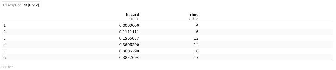
Given that the estimated cumulative hazard is a function of time (i.e., \(\hat{\Lambda}(t)\)), we can manually derive the stepwise discrete-time derivative for the estimated cumulative baseline hazard function (hazard) with respect to time. Utilizing our self-created derivative function from the prior section, we then applied a non-parametric smooth curve to both the estimated cumulative baseline hazard function and baseline hazard function. There are various smoothing techniques available, and for this analysis, we employed the ss() function from the npreg package. We specified different degrees of freedom (df argument) to create smooth splines for the two estimated baseline hazards.

# Calculate numerical derivative
deri <- finite_differences(x = bhest$time, y = bhest$hazard)
baselineHazard <- cbind(bhest, deri)
colnames(baselineHazard) <- c('CumulativeBaselineHazard', 'Time', 'BaselineHazard')

# Non-parametric smooth curve for estimating baseline hazard function over time
smoothBH <- ss(x = baselineHazard$Time, y = baselineHazard$BaselineHazard, df = 4)

# Non-parametric smooth curve for estimating cumulative baseline hazard function over time
smoothCBH <- ss(x = baselineHazard$Time, y = baselineHazard$CumulativeBaselineHazard, df = 6)

Dt_Plot <- data.frame('Time' = baselineHazard$Time, 
                      'BH' = baselineHazard$BaselineHazard, 
                      'smoothBH' = smoothBH$y, 
                      'CBH' = baselineHazard$CumulativeBaselineHazard, 
                      'smoothCBH' = smoothCBH$y)

After combining the smooth curves with the original estimated (cumulative) baseline hazard functions using the Time steps, we will use this combined dataset to visualize these two functions. Initially, we visualize the raw estimated (cumulative) baseline functions without applying smoothers, using different colors. Here, since the cumulative baseline hazard (\(\Lambda(t) \geq 0\)) and baseline hazard (\(0 \leq \lambda_{0}(t) \leq 1\)) are on different scales, we create a second y-axis for the cumulative baseline hazard. Therefore, it is necessary to construct a scale factor to map values from the scale of cumulative hazard to the scale of baseline hazard.

# Set up color for smooth curves
colors <- c("Baseline hazard" = "blue", "Cumulative baseline\nhazard" = "#FFA500")

# Create scale factor for second y-axis
scaleFactor <- max(Dt_Plot$BH) /  max(Dt_Plot$CBH)

# Create x and y labels
xlab <- seq(0, 1000, length.out = 11)
ylab <- seq(0, 0.04, length.out = 5)

# Create figure
p <- 
  ggplot(Dt_Plot, aes(x = Time)) + 
  geom_point(aes(y = BH, color = 'Baseline hazard'), size = 0.75, alpha = 0.3) + 
  geom_path(aes(y = BH, color = 'Baseline hazard')) + 
  geom_path(aes(y = CBH * scaleFactor, color = 'Cumulative baseline\nhazard')) + 
  geom_point(aes(y = CBH * scaleFactor, color = 'Cumulative baseline\nhazard'), size = 0.75, alpha = 0.3) + 
  labs(x = 'Time', y = 'Raw baseline hazard') + 
  scale_x_continuous(expand = c(0, 0.01), limits = c(0, 1000), breaks = xlab, labels = xlab) +
  scale_y_continuous(expand = c(0, 0.01), 
                     sec.axis = sec_axis(trans = ~ ./scaleFactor, name = "Raw cumulative baseline hazard")) + 
  scale_color_manual(values = colors) + 
  theme_bw() + 
  theme(panel.background = element_blank(),                    
        axis.line.x = element_line(),                               
        axis.line.y = element_line(),
        axis.text.x = element_text(color = "black", size = 7), 
        axis.text.y = element_text(color = 'black', size = 7),
        legend.title = element_blank())
p

In this figure, the estimated baseline hazard points are depicted in blue using the left y-axis, the estimated cumulative baseline hazard is depicted in orange using the right y-axis, and the x-axis represents the time. It is noteworthy that the relationship between the two estimated functions is such that the slope of the cumulative baseline hazard function at each time point actually reflects the value of the baseline hazard function at that specific time point. The raw estimated cumulative baseline hazard function appears smoother than the estimated baseline hazard function. Now we are going to visualize the smoothed version of these two functions.

# Create scale factor for second y-axis
scaleFactor <- max(Dt_Plot$smoothBH) /  max(Dt_Plot$smoothCBH)

# Create figure
p <- 
  ggplot(Dt_Plot, aes(x = Time)) + 
  geom_path(aes(y = smoothBH, color = 'Baseline hazard')) + 
  geom_path(aes(y = smoothCBH * scaleFactor, color = 'Cumulative baseline\nhazard')) + 
  labs(x = 'Time', y = 'Baseline hazard') + 
  scale_x_continuous(expand = c(0, 0), limits = c(0, 1000), breaks = xlab, labels = xlab) +
  scale_y_continuous(expand = c(0, 0), limits = c(0, 0.04), breaks = ylab, labels = round(ylab, 3), 
                     sec.axis = sec_axis(trans = ~ ./scaleFactor, name = "Cumulative baseline hazard")) + 
  scale_color_manual(values = colors) + 
  theme_bw() + 
  theme(panel.background = element_blank(),                    
        axis.line.x = element_line(),                               
        axis.line.y = element_line(),
        axis.text.x = element_text(color = "black", size = 7), 
        axis.text.y = element_text(color = 'black', size = 7),
        legend.title = element_blank())
p

In the smoothed version, the estimated cumulative baseline hazard function monotonically increases, while the estimated baseline hazard function reflects the baseline risk of secondary viral infections when there are no factors adjusted for. The risk of getting a secondary viral infection in the environment decreases initially, increases in the second stage, and eventually decreases again approaching the end of the study period. Since this is simulated data, the estimated baseline risk may not truly reflect respiratory viral interference in the environment. Sometimes, this estimated baseline risk can be verified by the smooth curve for the estimated incidence rate calculated from the same study.