This tutorial guides you through the process of creating contour plots using ggplot2. A contour plot is a type of visualization used to represent a 3-dimensional surface by projecting constant z values onto a 2-dimensional space. It provides a straightforward way to visualize complex 3-dimensional datasets in a simplified 2-dimensional format. To illustrate the usage of contour plots, we will use the volcano dataset from the rgl package.
1. Contour plot: line
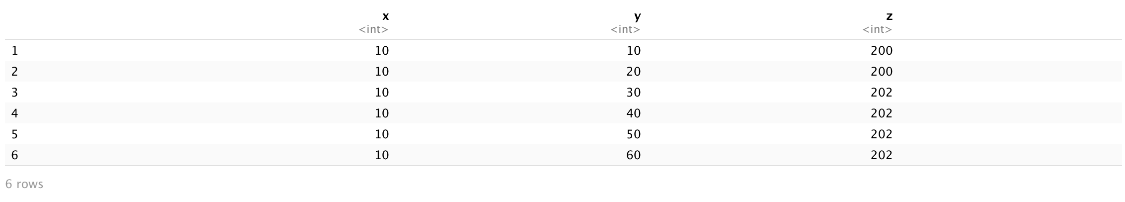
To illustrate the usage of contour plots, we will use the volcano dataset from the rgl package. The volcano dataset can be thought of as representing the longitudinal, latitudinal, and height data of a volcano. The longitudinal and latitudinal coordinates are presented by the x and y axes, respectively, while the height is represented by the z values in the matrix. This dataset consists of 87 rows and 61 columns, describing 5307 observations of the volcano’s topography. After data preprocessing, we will work with a subset of the dataset, including 3 columns for x, y, and z dimensions.
The data structure is simple, and we will first explore the line version of contour plots. In ggplot2, we primarily rely on two different functions: geom_contour() for contour plots.
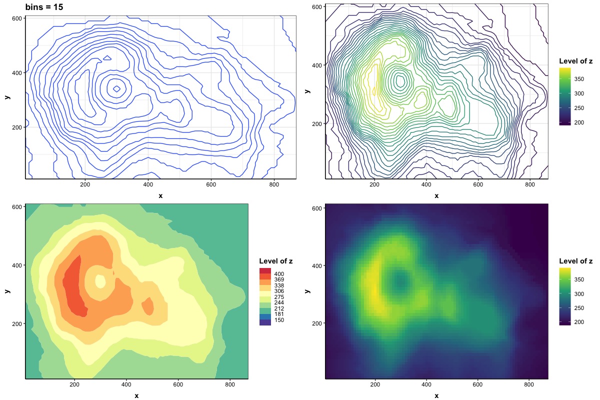
In the basic version of a contour plot, we have the ability to manage the number of bins to effectively visualize distinct contours within the same dataset. Each figure in this representation incorporates contour lines that faithfully reflect the underlying 3-dimensional data structure.
# Version 1
## bins = 15
p1 <-
ggplot(Dt, aes(x, y, z = z)) +
  geom_contour(bins = 15) +                 # Create contour plot with 15 bins
  ggtitle('bins = 15') +
  scale_x_continuous(expand = c(0, 0)) +
  scale_y_continuous(expand = c(0, 0)) +
  theme_bw() +                                                      # dark-on-light theme
  theme(panel.background = element_blank(),
        axis.line.x = element_line(),                               # these two are for the axis line
        axis.line.y = element_line(),
        axis.text.x = element_text(colour = "black"),               # there two are for texts in axes
        axis.text.y = element_text(colour = "black"),
        axis.ticks.x = element_line(),                              # these two are for ticks in axes
        axis.ticks.y = element_line(),
        axis.title.x = element_text(colour = "black", face = 'bold', vjust = -1),
        axis.title.y = element_text(colour = "black", face = 'bold'),
        plot.title = element_text(face = 'bold'),
        legend.title = element_text(colour = "black", face = 'bold'),
        legend.text = element_text(colour = "black"))

## bins = 30
p2 <-
ggplot(Dt, aes(x, y, z = z)) +
  geom_contour(bins = 30) +                # Create contour plot with 30 bins
  ggtitle('bins = 30') +
  scale_x_continuous(expand = c(0, 0)) +
  scale_y_continuous(expand = c(0, 0)) +
  theme_bw() +                                                      # dark-on-light theme
  theme(panel.background = element_blank(),
        axis.line.x = element_line(),                               # these two are for the axis line
        axis.line.y = element_line(),
        axis.text.x = element_text(colour = "black"),               # there two are for texts in axes
        axis.text.y = element_blank(),
        axis.ticks.x = element_line(),                              # these two are for ticks in axes
        axis.ticks.y = element_line(),
        axis.title.x = element_text(colour = "black", face = 'bold', vjust = -1),
        axis.title.y = element_blank(),
        plot.title = element_text(face = 'bold'),
        legend.title = element_text(colour = "black", face = 'bold'),
        legend.text = element_text(colour = "black"))

# Arrange 2 figures
Layout.Mat <- matrix(c(rep(1, 9), rep(2, 8)), nrow = 1)
grid.arrange(p1, p2, layout_matrix = Layout.Mat)
.jpeg)
We observe that increasing the number of bins results in a denser figure. Although the transformation from 3-dimensional data to a 2-dimensional representation provides a general shape of the data, it doesn’t fully capture the original range of continuous variable z. Therefore, in the upcoming version, our aim is to visualize the magnitude of the continuous z using a contour plot. In the default configuration of geom_contour(), two intermediate values are calculated: level_mid (a numerical value corresponding to the midpoint of the contour levels) and level (an ordered factor representing the contour range). Hence, it becomes necessary to utilize the after_stat() function in ggplot2. This function enables us to extract and utilize variables that have been calculated by the stat.
# Version 2
p3 <-
ggplot(Dt, aes(x, y, z = z)) +
  geom_contour(aes(colour = after_stat(level)), bins = 30) +       # Create contour plot with 30 bins and set color of level
  scale_color_continuous(type = 'viridis') +
  ggtitle('bins = 30') +
  scale_x_continuous(expand = c(0, 0)) +
  scale_y_continuous(expand = c(0, 0)) +
  theme_bw() +                                                      # dark-on-light theme
  theme(panel.background = element_blank(),
        axis.line.x = element_line(),                               # these two are for the axis line
        axis.line.y = element_line(),
        axis.text.x = element_text(colour = "black"),               # there two are for texts in axes
        axis.text.y = element_text(colour = "black"),
        axis.ticks.x = element_line(),                              # these two are for ticks in axes
        axis.ticks.y = element_line(),
        axis.title.x = element_text(colour = "black", face = 'bold', vjust = -1),
        axis.title.y = element_text(colour = "black", face = 'bold'),
        plot.title = element_text(face = 'bold'),
        legend.title = element_text(colour = "black", face = 'bold'),
        legend.text = element_text(colour = "black"))

# Modify legend title
p3$labels$colour <- 'Level of z'
p3
.jpeg)
In this version, the contour line values are color-coded using a continuous color scale. Bright colors signify higher magnitudes of z, while darker colors represent lower magnitudes of z. Instead of visualizing contours solely with lines, we can also represent them using color-filled areas or tiles which we will explore in the next section.
2. Contour plot: tile
To create a contour plot with color-filled areas or tiles, we mainly utilize two functions: geom_contour_filled() or geom_raster(). In this section, we’ll introduce the usage of geom_contour_filled(), which closely resembles geom_contour(). However, unlike controlling the number of bins with geom_contour_filled(), we modify the tile version of the contour plot by adjusting the number of breaks within the range of z values. The breaks argument, when supplied to geom_contour_filled(), serves the purpose of defining a numerical vector of breaks to segment the z range into distinct sub-intervals, each represented by a unique color. To enhance the creation of a divergent color palette, we will employ a function, namely brewer.pal(), from the RColorBrewer package. The brewer.pal() function take two arguments:
Once we’ve chosen a color palette, we can apply it by passing it to scale_fill_manual() in order to manually set the color palette for the color-filled tiles within the contour plot. The generated color palette is assigned to the values argument, and we use drop = F to ensure that unused factor levels are not dropped by the function. Additionally, we utilize the guide_colorsteps() function within the guides() function to ensure the color legend is displayed vertically (guide_colorsteps(direction = "vertical")). In general, guides() function is used to modify different scales (i.e., color, fill, legend, etc.) in ggplot2.
# Create selected palette
require(RColorBrewer)
Breaks <- c(-Inf, seq(150, 400, length.out = 9), Inf)               # set up the number of breaks
Spectral.colors <- brewer.pal(n = length(Breaks), name = "Spectral") # generate color palette

# Version 3
p4 <-
ggplot(Dt, aes(x, y, z = z)) +
  geom_contour_filled(breaks = Breaks) +            # pass Breaks (approximately bins = 11)
  scale_fill_manual(values = rev(Spectral.colors),  # set up color palette manually and using decrasing order for values
                    drop = F) +                     # avoid dropping unused factors
  guides(fill = guide_colorsteps(direction = "vertical")) +         # vertically display legend
  scale_x_continuous(expand = c(0, 0)) +
  scale_y_continuous(expand = c(0, 0)) +
  theme_bw() +                                                      # dark-on-light theme
  theme(panel.background = element_blank(),
        axis.line.x = element_line(),                               # these two are for the axis line
        axis.line.y = element_line(),
        axis.text.x = element_text(colour = "black"),               # there two are for texts in axes
        axis.text.y = element_text(colour = "black"),
        axis.ticks.x = element_line(),                              # these two are for ticks in axes
        axis.ticks.y = element_line(),
        axis.title.x = element_text(colour = "black", face = 'bold', vjust = -1),
        axis.title.y = element_text(colour = "black", face = 'bold'),
        plot.title = element_text(face = 'bold'),
        legend.title = element_text(colour = "black", face = 'bold'),
        legend.text = element_text(colour = "black"))

# Modify legend title
p4$labels$fill <- 'Level of z'
p4
.jpeg)
In this version of the contour plot, each area represented by contour lines from geom_contour() is now filled with different colors from a continuous color scale. When compared to the line version of the contour plot, the tile version is likely to be more intuitive. Another alternative to the geom_contour_filled() function is to combine the use of geom_raster() and geom_contour(). The geom_raster() function is particularly useful when all the tiles are of the same size, offering high performance. In this context, each tile in a contour plot corresponds to a rectangle or square, and colors are applied to fill each tile to represent the mapping of the ‘z’ values onto a 2-dimensional grid.
# Version 4
p5 <-
ggplot(Dt, aes(x, y, z = z)) +
  geom_contour(bins = 11) +            # create contour plot with 30 bins and set color of level
  geom_raster(aes(fill = z)) +         # fill grid
  scale_fill_continuous(type = 'viridis') +
  ggtitle('bins = 11') +
  scale_x_continuous(expand = c(0, 0)) +
  scale_y_continuous(expand = c(0, 0)) +
  theme_bw() +                                                      # dark-on-light theme
  theme(panel.background = element_blank(),
        axis.line.x = element_line(),                               # these two are for the axis line
        axis.line.y = element_line(),
        axis.text.x = element_text(colour = "black"),               # there two are for texts in axes
        axis.text.y = element_text(colour = "black"),
        axis.ticks.x = element_line(),                              # these two are for ticks in axes
        axis.ticks.y = element_line(),
        axis.title.x = element_text(colour = "black", face = 'bold', vjust = -1),
        axis.title.y = element_text(colour = "black", face = 'bold'),
        plot.title = element_text(face = 'bold'),
        legend.title = element_text(colour = "black", face = 'bold'),
        legend.text = element_text(colour = "black"))
# Modify legend title
p5$labels$fill <- 'Level of z'
p5
.jpeg)
This version of the contour plot conveys the same level of information as the one mentioned earlier. The key distinction in this version lies in the discretization of the continuous x and y axes into a grid of uniform size. Each grid cell is then filled with a color corresponding to the value of z.